Pages

Thursday, July 9, 2015

The Ecology of Local Subspaces: Mixtures of Parochial Views

No matter where you live, your view of the world is biased and limited, which is the beauty of this magazine cover.


As a marketer, of course, all my maps depict, not place, but consumption. For example, in an earlier post I asked, "What apps are on your Smartphone?" It seemed like a reasonable question for a marketing researcher interested in cross-selling or just learning more about product usage. Nothing special about apps, the same question could have been raised about movies, restaurants, places you drive your car, or stuff that you buy using your credit card. In all these cases, there is more available than any one consumer will use or know. Regardless of what or how we consume, our awareness and familiarity will have the parochial feel of the New Yorker cartoon.

Not Really Big Data But Too Much for a Single Bite

Because we are surveying consumers, we are unlikely to collect data from more than a few thousand respondents, and there are limits to how much information we can obtained before they stop responding. This is not Netflix ratings or Facebook friending or Google searches. Still, the "world of apps" for the young teen in school and the business person using their phone for work are too distant to analyze in a single bite. Moreover, these worldviews cannot be disentangled by examining marginal row or column effects alone for they are a mixture of local subspaces defined by the joint clustering of rows and columns together.

I have titled this post "The Ecology of Local Subspaces" in the hope that our knowledge of ecological systems will help us understand consumption. Animals are mobile, yet the features that enable the movement of fish, birds, and mammals tend to be distinct since they inhabit different subspaces. Hoofed animals are not more or less similar because they do not have wings or fins. Two individuals are similar if they have the same apps on their Smartphones only after we have identified the local subspace of relevant apps that define their similarity. Same and different have meaning only within a given frame of reference. Different apps will enter the similarity computations for those with differing worldviews determined by their situation and usage patterns. An earlier post provides a more detail account and suggests several R packages for simultaneous clustering.

Matrix Factorization Yields a Single Set of Joint Latent Factors 

I have already rejected the traditional approach of marginal row and column clustering. That is, one could cluster the rows using all the columns to calculate distances, either a distance matrix for all the rows or distances to proposed cluster centroids as in k-means clustering. Nothing forces us to make these distances Euclidean, and there are other distance measures in R. The same clustering could be attempted for the columns, although some prefer a factor analysis if they can obtain a reasonable correlation matrix given the columns are binary and sparse.

Our focus, however, is on the matrix whose block pattern is determined by the joint action of the rows and columns together. We seek a single set of joint latent factors with row contributions and column weights that reproduce the data matrix when their product is formed. What forces are at work in the Smartphone apps market that might generate such local subspaces? One could see our joint latent factors as the result of the need to accomplish desired tasks. Then, the apps co-reside on the same Smartphone because together they accomplish those desired tasks, and users who want to perform those tasks receive high scores on the corresponding joint latent factor.

Suppose that we start with 1000 respondents and 100 apps to form a 1000 x 100 data matrix with 100,000 data points (1000 x 100 = 100,000). Finding 10 joint latent factors would mean that we could approximate the 100,000 data points by multiplying a 1000 x 10 user factor score matrix times a 10 x 100 apps factor loading matrix. The matrix multiplication would look like the following diagram (except for more rows and columns for all three matrices) with W containing the 10 factor scores for the 1000 users and H holding the 10 sets of factor loadings for the 100 apps.
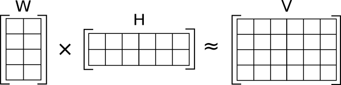

The data reduction is obvious given that before I needed 100 apps indicators to describe a user, now I need only 10 joint latent factor scores. Clearly, in order to reproduce the original data matrix, we will require the factor loadings telling us which apps load on which joint latent factors.

More importantly, we will have made the representation simpler by naming the joint latent factors responsible for the data reduction. Apps are added for a purpose, in fact, multiple apps may be installed together or over time to achieve a common goal. The coefficient matrix H displays those purposes as the joint latent factors and the apps that serve those purposes as the factor loadings in each row. The simplification is complete with W that describes the users in terms of those purposes or joint latent factors and not by a listing of the original 100 apps. 

Our hope is to discover an underlying structure revealing the hidden forces generating the observed usage patterns across diverse user communities.

Monday, July 6, 2015

Regression with Multicollinearity Yields Multiple Sets of Equally Good Coefficients

The multiple regression equation represents the linear combination of the predictors with the smallest mean-squared error. That linear combination is a factorization of the predictors with the factors equal to the regression weights. You may see the words "factorization" and "decomposition" interchanged, but do not be fooled. The QR decomposition or factorization is the default computational method for the linear model function lm() in R. We start our linear modeling by attempting to minimize least square error, and we find that a matrix computation accomplishes this task fast and accurately. Regression is not unique for matrix factorization is a computational approach that you will rediscover over and over again as you add R packages to your library (see Two Purposes for Matrix Factorization).

Now, multicollinearity may make more sense. Multicollinearity occurs when I have included in the regression equation several predictors that share common variation so that I can predict any one of those predictors from some linear combination of the other predictors (see tolerance in this link). In such a case, it no longer matters what weights I give individual predictors for I get approximately the same results regardless. That is, there are many predictor factorizations yielding approximately the same predictive accuracy. The simplest illustration is two highly correlated predictors for which we obtain equally good predictions using any one predictor alone or any weighted average of the two predictors together. "It don't make no nevermind" for the best solution with the least squares coefficients is not much better than the second best solution or possibly even the 100th best solution. Here, the "best" solution is defined only for this particular dataset before we ever begin to talk about cross-validation.

On the other hand, when all the predictors are mutually independent, we can speak unambiguously about the partitioning of R-squared. Each independent variable makes its unique contribution, and we can simply add their impacts for the total is truly the sum of the parts. This is the case with orthogonal experimental designs where one calculates the relative contribution of each factor, as one does in rating-based conjoint analysis where the effects are linear and additive. However, one needs to be careful when generalizing from rating-based to choice-based conjoint models. Choice is not a linear function of utility so that the impact on share from changing any predictor depends on the values of all the predictors, including the predictor being manipulated. Said differently, the slope of the logistic function is not constant but varies with the values of the predictors.

We will ignore nonlinearity in this post and concentrate on non-additivity. Our concern will be the ambiguity that enters when the predictors are correlated (see my earlier post on The Relative Importance of Predictors for a more complete presentation).

The effects of collinearity are obvious from the formula calculating R-squared from the cells of the correlation matrix between y and the separate x variables. With two predictors, as shown below by the subscripts 1 and 2, we see that R-squared is a complex interplay of the separate correlations of each predictor with y and the interrelationships among the predictors. Of course, everything simplifies when the predictors are independent with r(1,2)=0 and the numerator reducing to the sum of the squared correlations of each predictor with y divided by a denominator equal to one.


The formulas for the regression coefficients mirror the same "adjustment" process. If the correlation between the first predictor and y represents the total effect of the first variable on y, then the beta weight shows the direct effect of the first variable after removing the its indirect path through the second predictor. Again, when the predictors are uncorrelated, the beta weight equals the correlation with y.


We speak of this adjustment as controlling for the other variables in the regression equation. Since we have only two independent variables, we can talk of the effect of variable 1 on y controlling for variable 2. Such a practice seems to imply that the meaning of variable 1 has not been altered by the controlling for variable 2. We can be more specific by letting variable 1 be a person's weight, variable 2 be a person's height and the dependent variable be some measure of health. What is the contribution of weight to health controlling for height? Wait a second, weight controlling for height is not the same variable as weight. We have a term for that new variable; we call it obesity. Simply stated, the meaning of a term changes as move from the marginal (correlations) to conditional (partial correlations) representations.

None of this is an issue when our goal is solely prediction. Yet, the human desire to control and explain is great, and it is difficult to resist the temptation to jump from association to causal inference. The key is not to accept the data as given but to search for a representation that enables us to estimate additive effects. One alternative treats observed variables as the bases for latent variable regression in structural equation modeling. Another approach, nonnegative matrix factorization (NMF), yields a representation in terms of building blocks that can additively be combined to form relatively complex structures. The model does not need to be formulated as a matrix factorization problem in order for these computational procedures to yield solutions.

Friday, July 3, 2015

The Nature of Heterogeneity in Coevolving Networks of Customers and Products

The genre shirt asks, "What kind of music do u listen 2?"

Microgenres exist because markets are fragmenting and marketers need names to attract emerging customer segments with increasingly specific preferences. The cost of producing and delivery music now supports a plenitude of joint pairings of recordings and customers. The coevolution of music and its audience binds together listening preferences and available alternatives.

I already know a good deal about your preferences by simply knowing that you listen to German Hip Hop or New Orleans Jazz (see the website Every Noise at Once). Those microgenres are not accidental but were named in order to broadcast the information that customers need in order to find what they want to buy and at the same time that artists require to market their goods. Matchmaking demands its own vocabulary. Over time, the language adapts and only the "fittest" categories survive.

R Makes It Easy

The R package NMF simplifies the analysis as I demonstrated in my post on Modeling Plenitude and Speciation. Unfortunately, the data in that post were limited to only 17 broad music categories, but the R code would have been the same had there been several hundred microgenres or several thousand songs.

The output is straightforward once you understand what nonnegative matrix factorization (NMF) is trying to accomplish. All matrix factorizations, as the name implies, attempt to identify "simpler" matrices or factors that will reproduce approximately the original data matrix when multiplied together. Simpler, in this case, means that we replace the many observed variables with a much smaller number of latent variables. The belief is that these latent variables will simultaneously account for both row cliques and column microgenres as they coevolve.

This is the matrix factorization diagram that I borrowed from Wikipedia to illustrate the process.


The original data matrix V holds the non-negative numbers indicating the listening intensities for every microgenre is approximated by multiplying a customer graded membership matrix W times a matrix of factor loadings for the observed variables H. The columns of W and the rows of H reflect the number of latent variables. It can be argued that V contains noise so that reproducing it exactly would be overfitting. Thus, nothing of "true" value is lost by replacing the original observations in V with the customer latent scores in W. As you can see, W has fewer columns, but I can always approximate V using the factor loadings in H as a "decoder" to reconstitute the observations without noise (a form of data compression).

Interpreting the Output

We start our interpretation of the output with H containing the factor loadings for the observed variables. For example, we might expect to see one of the latent variables reflecting interest in classical music with sizable factor loadings for the microgenres associated with such music. One of these microgenre could serve as an "anchor" that defines this latent feature if only the most ardent classical music fans listened to this specific microgenre (e.g., Baroque). Hard rock or jazz might be anchors for other latent variables. If we have been careful to select observed variables with high imagery (e.g., is it easy to describe the hard rock listener?), we will be able to name the latent variable based only on its anchors and other high loadings.

The respondent matrix W serves a similar function for customers. Each column is the same latent variable we just described in our interpretation of H. For every row, W gives us a set of graded membership indices telling us the degree to which each latent variable contributes to that respondent's pattern of observed scores. The opera lover, for instance, would have a high membership index for the latent variable associated with opera. We would expect to find a similar pairing between the jazz enthusiasts and a jazz-anchored latent variable, assuming that this is the structure underlying the coevolving network of customer and product.

Once again, we need to remember that nonnegative matrix factorization attempts to reproduce the observed data matrix as closely as possible given the constraints placed on it by limiting the number of latent variables and requiring that all the entries be non-negative. The constraint on the number of latent variables should seem familiar to those who have some experience with principal component or factor analysis. However, unlike principal component analysis, NMF adds the restriction that all the elements of W and H must be non-negative. The result is a series of additive effects with latent variables defined as nonnegative linear combinations of observed variables (H) and respondents represented as convex combinations of those same latent variables (W). Moreover, latent variables can only add to the reproduced intensities as they attempt to approximate the original data matrix V. Lee and Seung explain this as "learning the parts of objects."

Why NMF Works with Marketing Data

All this works quite nicely in fragmented markets where products evolve along with customers desires to generate separate communities. In such coevolving networks, the observed data matrix tends to be sparse and requires a simultaneous clustering of rows and columns. The structure of heterogeneity or individual differences is a mixture of categories and graded category memberships. Customers are free to check as many boxes as they wish and order as much as they like. As a result, respondents can be "pure types" with only one large entry in their row of W and all the other values near zero, or they can be "hybrids" with several substantial membership entries in their row.

Markets will continue to fragment with customers in control and the internet providing more and more customized products. We can see this throughout the entertainment industry (e.g., music, film, television, books, and gaming) but also in almost everything online or in retail warehouses. Increasingly, the analyst will be forced to confront the high-dimensional challenge of dealing with subspaces or local regions populated with non-overlapping customers and products. Block clustering of row and columns is the first step when the data matrix is sparse because these variables over here are relevant only for those respondent over there. Fortunately, R provides the link to several innovative methods for dealing with such case (see my post The Ecology of Data Matrices). 


Sunday, June 28, 2015

Generalizing from Marketing Research: The Right Question and the Correct Analysis

The marketing researcher asks some version of the following question in every study, "Tell me what you want?" The rest is a summary of the notes taken during the ensuing conversation.


Steve Jobs' quote suggests that we might do better getting a reaction to an actual product. You tell me that price is not particularly important to you, yet this one here costs too much. You claim that design is not an issue, except you love the look of the product shown. In casual discussion color does not matter, but that shade of aqua is ugly and you will not buy it.

Although Steve Jobs was speaking of product design using focus groups, we are free to apply his rule to all decontextualized research. "Show it to them" provides the context for product design when we embed the showing within a usage occasion. On the other hand, if you seek incremental improvements to current products and services, you ask about problems experienced or extensions desired in concrete situations because that is the context within which these needs arise. Of course, we end up with a lot more variables in our datasets as soon as we start asking about the details of feature preference or product usage.

For example, instead of rating the importance of color in your next purchase of a car, suppose that you are shown a color array with numerous alternatives to which many of your responses are likely to be "no" or  marked "not applicable" because some colors are associated with options you are not buying. Yet, this is the context within which cars are purchased, and the manufacturer must be careful not to lose a customer when no color option is acceptable. In order to respond to the rating question, the car buyer searches memory for instances of "color problems" in the past. The manufacturer, on the other hand, is concerned about "color problems" in the future when only a handful of specific color combinations are available. Importance is simply the wrong question given the strategic issues.

Because the resulting data are high dimensional and sparse, it will be difficult to analyze with traditional multivariate techniques. This is where R makes it contribution by offering tools from machine and statistical learning designed for sparse and high dimensional data that are produced whenever we provide a context.

We find such analyses in the data from fragmented product categories, where diverse consumer segments shop within distinct distribution channels for non-overlapping products and features (e.g., music purchases by young teens and older retirees). We can turn to R packages for nonnegative matrix factorization (NMF) and matrix completion (softImpute) to exploit such fragmentation and explain the observed high-dimensional and sparse data in terms of a much smaller set of inferred benefits.

What does your car color say about you? It's a topic discussed in the media and among friends. It is a type of collaboration among purchasers who may have never met yet find themselves in similar situations and satisfy their needs in much the same manner. A particular pattern of color preferences has meaning only because it is shared by some community. Matrix factorization reveals that hidden structure by identifying the latent benefits responsible for the observed color choices.

I may be mistaken, but I imagine that Steve Jobs might find all of this helpful.

Monday, June 22, 2015

Looking for Preference in All the Wrong Places: Neuroscience Suggests Choice Model Misspecification

At its core, choice modeling is a utility estimating machine. Everything has a value reflected in the price that we are willing to pay in order to obtain it. Here are a collection of Smart Watches from a search of Google Shopping. You are free to click on any one, look for more, or opt out altogether and buy nothing.


Where is the utility? It is in the brand name, the price, the user ratings and any other feature that gets noticed. If you pick only the Apple Smartwatch at its lowest price, I conclude that brand and price have high utility. It is a somewhat circular definition: I know that you value the Apple brand because you choose it, and you pick the Apple watch because the brand has value. We seem to be willing to live with such circularity as long as utility measured in one setting can be generalized over occasions and conditions. However, context matters when modeling human judgment and choice, making generalization a difficult endeavor. Utility theory is upended when higher prices alter perceptions so that the same food tastes better when it costs more.

What does any of this have to do with neuroscience? Utility theory was never about brain functioning. Glimcher and Fehr make this point in their brief history of neuroeconomics. Choice modeling is an "as if" theory claiming only that decision makers behave as if they assigned values to features and selected the option with the optimal feature mix.

When the choice task has been reduced to a set of feature comparisons as is the common practice in most choice modeling, the process seems to work at least in the laboratory (i.e., care must be taken to mimic the purchase process and adjustment may be needed when making predictions about real-world market shares). Yet, does this describe what one does when looking at the above product display from Google Shopping? I might try to compare the ingredients listed on the back of two packages while shopping in the supermarket. However, most of us find this task quickly becomes too difficult as the number of features exceeds our short-term memory limits (paying attention is costly).

Incorporating Preference Construction

Neuroeconomics suggests how value is constructed on-the-fly in real world choice tasks. Specifically, reinforcement learning is supported by multiple systems within the brain: "dual controllers" for both the association of features and rewards (model-free utilities) and the active evaluation of possible futures (model-based search). Daw, Niv and Dayan identified the two corresponding regions of the brain and summarized the supporting evidence back in 2005.

Features can become directly tied to value so that the reward is inferred immediately from the presence of the feature. Moreover, if we think of choice modeling only as the final stages when we are deciding among a small set of alternatives in a competitive consideration set, we might mistakenly conclude that utility maximization describes decision making. As in the movies, we may wish to "flashback" to the beginning of the purchase process to discover the path that ended at the choice point where features seem to dominate the representation.

Perception, action and utility are all entangled in the wild, as shown by the work of Gershman and Daw. Attention focuses on the most or least desirable features in the context of the goals we wish to achieve. We simulate the essentials of the consumption experience and ignore the rest. Retrospection is remembering the past, and prospection is experiencing the future. The steak garners greater utility sizzling than raw because it is easier to imagine the joy of eating it.

While the cognitive scientist wants to model the details of this process, the marketer will be satisfied learning enough to make the sale and keep the customer happy. In particular, marketing tries to learn what attracts attention, engages interest and consideration, generates desire and perceived need, and drives purchase while retaining customers (i.e., the AIDA model). These are the building blocks from which value is constructed.

Choice modeling, unfortunately, can identify the impact of features only within the confines of a single study, but it encounters difficulties attempting to generalize any effects beyond the data collected. Many of us are troubled that even relatively minor changes can alter the framing of the choice task or direct attention toward a previously unnoticed aspect (Attention and Reference Dependence).

The issue is not one of data collection or statistical analysis. The R package support.BWS will assist with the experimental design, and other R packages such as bayesm, RSGHB and ChoiceModelR will estimate the parameters of a hierarchical Bayes model. No, the difficulty stems from needing to present each respondent with multiple choice scenarios. Even if we limit the number of choice sets that any one individual will evaluate, we are still forced to simplify the task in order to show all the features for all the alternatives in the same choice set. In addition, multiple choice sets impose some demands for consistency so that a choice strategy that can be used over and over again without a lot of effort is preferred by respondents just to get through the questionnaire. On the other hand, costly information search is eliminated, and there is no anticipatory regret or rethinking one's purchase since there is no actual transfer of money. In the end, our choice model is misspecified for two reasons: it does not include the variables that drive purchase in real markets and the reactive effects of the experimental arrangements create confounding effects that do not occur outside of the study.

Measuring the Forces Shaping Preference

Consumption is not random but structured by situational need and usage occasion. "How do you intend to use your Smartwatch?" is a good question to ask when you begin your shopping, although we will need to be specific because small differences in usage can make a large difference in what is purchased. To be clear, we are not looking for well-formed preferences, for instance, feature importance or contribution to purchase. Instead, we focus on attention, awareness and familiarity that might be precursors or early phases of preference formation. If you own an iPhone, you might never learn about Android Wear. What, if anything, can we learn from the apps on your Smartphone?

I have shown how the R package NMF for nonnegative matrix factorization can uncover these building blocks. We might wish to think of NMF as a form of collaborative filtering, not unlike a recommender system that partitions users into cliques or communities and products into genres or types (e.g., sci-fi enthusiasts and the fantasy/thrillers they watch). An individual pattern of awareness and familiarity is not very helpful unless it is shared by a larger community with similar needs arising from common situations. Product markets evolve over time by appealing to segments willing to pay more for differentiated offerings. In turn, the new offerings solidify customer differences. This separation of products and users into segregated communities forms the scaffolding used to construct preferences, and this is where we should begin our research and statistical analysis.

Tuesday, June 2, 2015

Statistical Models with a Point of View: First vs. Third Person


Marketing data can be collected in the first or third person, and we require different statistical models for each point of view.


Netflix encourages you to adopt a third-person perspective when it surveys your taste preferences by asking how often you watch different genres (e.g., action and adventures, comedies, dramas, horror, thrillers and more). Third-person remembering taps those regions of the brain responsible for semantic memory. We respond as we would in a conversation providing general information about ourselves. Is the Twilight Saga horror or romance? It does not matter since we answer about the genre without retrieving specific movies. Neither do we ponder the definition of the response categories: never, sometimes and often. I never watch horror films because they scare me and I avoid them, which I should not know because I never watch them, except for the horror movies that I do see and call thrillers. Such preference ratings are positioning statements about who we think we are and how we wish to present ourselves.

On the other hand, first-person recollection is needed to rate individual movies that we have seen. We answer by reliving the viewing experience, which is impacted by context (where, when, who we were with and what else we were doing while watching). We call this episodic memory, which is different from semantic memory, with its own region of the brain and its own retrieval process. Someone asks if you liked a particular movie and you cannot remember seeing it until they tell you the actors and describe aspects of the plot. Both of these are examples of episodic memory. First, the movie that was a blur suddenly becomes clear after some detail is mentioned and memories flood your mind. The second example is your first-person recollection that you have had such an episodic memory experience in the past.

We analyze data obtained from third-person remembering using the statistical methods that are most familiar to those with a social science background (e.g., regression, factor analysis and structural equation modeling). Semantic data is, well, semantic, and it has a factor structure that reflects the meaning of words. If you say that you like action films, then any genre associated with action will also be liked, where association is found in the way words are used by marketers, film critics and in everyday conversation. If I mention Jurassic Park, one can bring to mind one or more scenes from the film and perhaps even recall some details about your first viewing. You cannot do the same for the "science fiction" category, assuming that Jurassic Park is science fiction and not fantasy/thriller.

My point is that any questions about the genre or category will be answered by retrieving general semantic knowledge, including the way we have learned to talk about those genres. Thus, if I ask about usage, satisfaction or importance, I will be tapping the same semantic knowledge structures with all the relationships that you have learned over time by telling others what you think and feel and listening to others tell you what they think and feel. It will not matter whether my measurement is a rating or some type of tradeoff or ranking (e.g., MaxDiff). I am not denying that such information is useful to marketing simply that it is at least one step removed from remembered experiences.

This is not the case with first-person recollection that forces the respondent to relive the episode. You recently watched a specific movie and now you give it a rating by remembering how you felt and how much you liked it. Over time you can rate many movies, but only a very small fraction of all that is available. Your movie rating data is high-dimensional and sparse. Moreover, this tends to be the case for episodic data in general when the episodes are occasion-based combinations of many factors (e.g., who uses what for this or that purpose at a particular time in a specific place with or without others present).

In the third-person, we can ask everyone the same question and let them fill in the details. "How important was product quality when you made your purchase?" deliberatively leaves product quality open to interpretation. But in the first-person we ask about a series of specific events: knowing warranty protection and return policy, reviewing user comments, reading expert evaluations, trial usage in a store or through another user, familiarity with the brand, and so on. Of course, product quality is but one of many purchase criteria, so the list of specific events gets quite long and increasingly sparse since potential customers tend to focus their attention on a subset of all the items in our checklist.

As sparse data become more common, R adds more ways to handle it with both supervised (glmnet) and unsupervised (sparcl) packages. The new book by Hastie, Tibshirani and Wainwright, Statistical Learning with Sparsity, brings together all this work along with matrix decomposition and compressed sensing (which is where one would place nonnegative matrix factorization). High dimensionality ceases to be a curse and turns into a blessing when the additional data reveals an underlying structure that we could not observe until we began to ask in the first person.

Saturday, May 30, 2015

Top of the Heap: How Much Can We Learn from Partial Rankings?

The recommendation system gives you a long list of alternatives, but the consumer clicks on only a handful: most appealing first, then the second best, and so on until they stop with all the remaining receiving the same rating as not interesting enough to learn more. As a result, we know the preference order for only the most preferred. Survey research may duplicate this process by providing many choices and asking only for your top three selections - your first, second and third picks. This post will demonstrate that by identifying clusters with different ranking schemes (mixtures of rankings), we can learn a good deal about consumer preferences across all the alternatives from observing only a limited ordering of the most desired (partial top-K rankings).

However, we need to remain open to the possibility that our sample is not homogeneous but contains mixtures of varying ranking schemes. To be clear, the reason for focusing on the top-K rankings is because we have included so many alternatives that no one person will be able to respond to all of them. For example, the individual is shown a screen filled with movies, songs, products or attributes and asked to pick the best of the list in order of preference. Awareness and familiarity will focus attention on some subset, but not the same subset for everyone. We should recall that N-K of the possible options will not be selected and thus be given zeros. Consequently, with individuals in rows and alternatives as columns, no one should be surprised to discover that the data matrix has a blockcluster appearance (as in the R package with the same name).
To see how all this works in practice, we begin by generating complete ranking data using the simulISR( ) function from the R package Rankcluster. The above graphic, borrowed from Wikipedia, illustrates the Insertion Sort Ranking (ISR) process that Rankcluster employs to simulate rankings. We start with eight objects in random order and sort them one at a time in a series of paired comparisons. However, the simulation function from Rankcluster allows us to introduce heterogeneity by setting a dispersion parameter called pi. That is, we can generate a sample of individuals sharing a common ranking scheme, yet with somewhat different observed rankings from the addition of an error component.

As an example, everyone intends to move #7 to be between #6 and #8, but some proportion of the sample may make "mistakes" with that proportion controlled by pi. Of course, the error could represent an overlap in the values associated with #6 and #7 or # 7 and #8 so that sometimes one looks better and other times it seems the reverse (sensory discrimination). Regardless, we do not generate a set of duplicate rankings. Instead, we have a group of ranks distributed about a true rank. The details can be found in their technical paper.

You will need to install the Rankcluster and NMF packages in order to run the following R code.

# Rankcluster needed to simulate rankings
library(Rankcluster)
 
# 100 respondents with pi=0.90
# who rank 20 objects from 1 to 20
rank1<-simulISR(100, 0.90, 1:20)
 
# 100 respondents with pi=0.90
# who rank 20 object in reverse order
rank2<-simulISR(100, 0.90, 20:1)
 
# check the mean rankings
apply(rank1, 2, mean)
apply(rank2, 2, mean)
 
# row bind the two ranking schemes
rank<-rbind(rank1,rank2)
 
# set ranks 6 to 20 to be 0s
top_rank<-rank
top_rank[rank>5]<-0
 
# reverse score so that the
# scores now represent intensity
focus<-6-top_rank
focus[focus==6]<-0
 
# use R package NMF to uncover
# mixtures with different rankings
library(NMF)
fit<-nmf(focus, 2, method="lee", nrun=20)
 
# the columns of h transposed
# represent the ranking schemes
h<-coef(fit)
round(t(h))
 
# w contains the membership weights
w<-basis(fit)
 
# hard clustering
type<-max.col(w)
 
# validates the mixture model
table(type,c(rep(1,100),rep(2,100)))

Created by Pretty R at inside-R.org

We begin with the simulIST( ) function simulating two sets of 100 rankings each. The function takes three arguments: the number of rankings to be generated, the value of pi, and the rankings listed for each object. The sequence 1:20 in the first ranking scheme indicates that there will be 20 objects ordered from first to last. Similarly, the sequence 20:1 in the second ranking scheme inputs 20 objects ranked in reverse from last to first. We concatenate data produced by the two ranking schemes and set three-quarters of the rankings to 0 as if only the top-5 rankings were provided. Finally, the scale is reversed so that the non-negative values suggest greater intensity with five as the highest score.

The R package NMF performs the nonnegative matrix factorization with the number of latent features set to two, the number of ranking schemes generating the data. I ask that you read an earlier post for the specifics of how to use the R package NMF to factor partial top-K rankings. More generally though, we are inputting a sparse data matrix with zeros filling 75% of the space. We are trying to reproduce that data (labeled V in the diagram below) by multiplying two matrices. One has a row for every respondent (w in the R code), and the other has a column for every object that was ranked (h in the R code). What links these two matrices is the number of latent features, which in this case happens also to be two because we simulated and concatenated two ranking schemes.


Let us say that we placed 20 bottles of wine along a shelf so that the cheapest was in the first position on the left and the most expensive was last on the shelf on the far right. These are actual wines so that most would agree that the higher priced bottles tended to be of higher quality. Then, our two ranking schemes could be called "price sensitivity" and "demanding palette" (feel free to substitute less positive labels if you prefer). If one could only be Price Sensitive or Demanding Palette and nothing in between, then you would expect precisely 1 to 20 and 20 to 1 rankings for everyone in each segment, respectively, assuming perfect knowledge and execution. That is, some of our drinkers may be unaware that #16 received a higher rating than #17 or simply give it the wrong rank. This is encoded in our pi parameter (pi=0.90 in this simulation). Still, if I knew your group membership and the bottle's position, I could predict your ranking with some degree of accuracy varying with pi.

Nonnegative matrix factorization (NMF) seeks to recover the latent features separating the wines and the latent feature membership for each drinker from the data matrix, which you recall does not contain complete rankings but only the partial top-K. Since I did not set the seed, your results will be similar, but not identical, to the following decomposition.

Columns
h
Demanding Palette
Price Sensitivity
Rows
w
Demanding Palette
Price Sensitivity
C1
0
368
R1
0.00000
0.01317
C2
0
258
R2
0.00100
0.00881
C3
0
145
R3
0.00040
0.00980
C4
4
111
R4
0.00105
0.00541
C5
18
68
R5
0.00000
0.01322
C6
49
80
R6
0.00000
0.01207
C7
33
59
R7
0.00291
0.00541
C8
49
61
R8
0.00361
0.00416
C9
45
50
R9
0.00242
0.01001
C10
112
31
.
.
.
C11
81
30
.
.
.
C12
63
9
.
.
.
C13
79
25
R193
0.01256
0.00000
C14
67
18
R194
0.00366
0.00205
C15
65
28
R195
0.01001
0.00030
C16
79
28
R196
0.00980
0.00000
C17
85
14
R197
0.00711
0.00028
C18
93
5
R198
0.00928
0.00065
C19
215
0
R199
0.01087
0.00000
C20
376
0
R200
0.01043
0.00000

The 20 columns from transposed h are presented first, and then the first few rows followed by the last rows from w. These coefficients will reproduce the data matrix, which contains numbers from 0 to 5. For instance, the reproduced score for the first respondent for the first object is 0*0.00000 + 386*0.01317 = 4.84656 or almost 5, suggesting that they most prefer the cheapest wine. In a similar fashion, the last row, R200, gives greater weight to the first column, and the first column seems to prefer the higher end of the wine continuum.

Clearly, there are some discrepancies toward the middle of the wine rankings, yet the ends are anchored. This makes sense given that we have data only on the top-5 rankings. Our knowledge of the ten objects in the middle comes solely from the misclassification when making pairwise comparisons set by pi=0.90. In the aggregate we seem to be able to see some differentiation even when we did not gather any individual data after the Kth position. Hopefully, C1 represents wine in a box and C20 is a famous vintage from an old village with a long wine history, making our interpretation of the latent features easier for us.

When I run this type of analysis with actual marketing data, I typically uncover many more latent features and find respondents with sizable membership weightings spread across several of those latent features. Preference for wine is based on more than a price-quality tradeoff, so we would expect to see other latent features accounting for the top-5 rankings (e.g., the reds versus the whites). The likelihood that an object makes it into the top-5 selection is a decreasing function of its rank order across the entire range of options so that we might anticipate some differentiate even when the measurement is as coarse as a partial ranking. NMF will discover that decomposition and reproduce the original rankings as I have shown with the above example. It seems that there is much we can learn for partial rankings.