
As a marketer, of course, all my maps depict, not place, but consumption. For example, in an earlier post I asked, "What apps are on your Smartphone?" It seemed like a reasonable question for a marketing researcher interested in cross-selling or just learning more about product usage. Nothing special about apps, the same question could have been raised about movies, restaurants, places you drive your car, or stuff that you buy using your credit card. In all these cases, there is more available than any one consumer will use or know. Regardless of what or how we consume, our awareness and familiarity will have the parochial feel of the New Yorker cartoon.
Not Really Big Data But Too Much for a Single Bite
Because we are surveying consumers, we are unlikely to collect data from more than a few thousand respondents, and there are limits to how much information we can obtained before they stop responding. This is not Netflix ratings or Facebook friending or Google searches. Still, the "world of apps" for the young teen in school and the business person using their phone for work are too distant to analyze in a single bite. Moreover, these worldviews cannot be disentangled by examining marginal row or column effects alone for they are a mixture of local subspaces defined by the joint clustering of rows and columns together.
I have titled this post "The Ecology of Local Subspaces" in the hope that our knowledge of ecological systems will help us understand consumption. Animals are mobile, yet the features that enable the movement of fish, birds, and mammals tend to be distinct since they inhabit different subspaces. Hoofed animals are not more or less similar because they do not have wings or fins. Two individuals are similar if they have the same apps on their Smartphones only after we have identified the local subspace of relevant apps that define their similarity. Same and different have meaning only within a given frame of reference. Different apps will enter the similarity computations for those with differing worldviews determined by their situation and usage patterns. An earlier post provides a more detail account and suggests several R packages for simultaneous clustering.
Matrix Factorization Yields a Single Set of Joint Latent Factors
I have already rejected the traditional approach of marginal row and column clustering. That is, one could cluster the rows using all the columns to calculate distances, either a distance matrix for all the rows or distances to proposed cluster centroids as in k-means clustering. Nothing forces us to make these distances Euclidean, and there are other distance measures in R. The same clustering could be attempted for the columns, although some prefer a factor analysis if they can obtain a reasonable correlation matrix given the columns are binary and sparse.
Our focus, however, is on the matrix whose block pattern is determined by the joint action of the rows and columns together. We seek a single set of joint latent factors with row contributions and column weights that reproduce the data matrix when their product is formed. What forces are at work in the Smartphone apps market that might generate such local subspaces? One could see our joint latent factors as the result of the need to accomplish desired tasks. Then, the apps co-reside on the same Smartphone because together they accomplish those desired tasks, and users who want to perform those tasks receive high scores on the corresponding joint latent factor.
Suppose that we start with 1000 respondents and 100 apps to form a 1000 x 100 data matrix with 100,000 data points (1000 x 100 = 100,000). Finding 10 joint latent factors would mean that we could approximate the 100,000 data points by multiplying a 1000 x 10 user factor score matrix times a 10 x 100 apps factor loading matrix. The matrix multiplication would look like the following diagram (except for more rows and columns for all three matrices) with W containing the 10 factor scores for the 1000 users and H holding the 10 sets of factor loadings for the 100 apps.
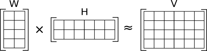
The data reduction is obvious given that before I needed 100 apps indicators to describe a user, now I need only 10 joint latent factor scores. Clearly, in order to reproduce the original data matrix, we will require the factor loadings telling us which apps load on which joint latent factors.
More importantly, we will have made the representation simpler by naming the joint latent factors responsible for the data reduction. Apps are added for a purpose, in fact, multiple apps may be installed together or over time to achieve a common goal. The coefficient matrix H displays those purposes as the joint latent factors and the apps that serve those purposes as the factor loadings in each row. The simplification is complete with W that describes the users in terms of those purposes or joint latent factors and not by a listing of the original 100 apps.
Our hope is to discover an underlying structure revealing the hidden forces generating the observed usage patterns across diverse user communities.
No comments:
Post a Comment