Customer Segmentation Using Purchase History: Another Example of Matrix Factorization

As promised in my last post, I am following up with another example of how to perform market segmentations with nonnegative matrix factorization. Included with the R package bayesm is a dataset called Scotch containing the purchase history for 21 brands of whiskey over a one year time period from 2218 respondents. The brands along with some features and pricing are listed below. You should note the column with the heading # Users, in particular, that the most to least popular brands vary from more than 36% to less than 2%.

#	Symbol	Brand	# Users	Price	Bottled	Type
1	CHR	Chivas Regal	806	21.99	Abroad	Blend
2	DWL	Dewar’s White Label	517	17.99	Abroad	Blend
3	JWB	Johnnie Walker Black	502	22.99	Abroad	Blend
4	JaB	J&B	458	18.99	Abroad	Blend
5	JWR	Johnnie Walker Red	424	18.99	Abroad	Blend
6	OTH	Other brands	414
7	GLT	Glenlivet	354	22.99	Abroad	Single malt
8	CTY	Cutty Sark	339	15.99	Abroad	Blend
9	GFH	Glenfiddich	334	39.99	Abroad	Single malt
10	PCH	Pinch (Haig)	117	24.99	Abroad	Blend
11	MCG	Clan MacGregor	103	10	US	Blend
12	BAL	Ballantine	99	14.9	Abroad	Blend
13	MCL	Macallan	95	32.99	Abroad	Single malt
14	PAS	Passport	82	10.9	US	Blend
15	BaW	Black & White	81	12.1	Abroad	Blend
16	SCY	Scoresby Rare	79	10.6	US	Blend
17	GRT	Grant’s	74	12.5	Abroad	Blend
18	USH	Ushers	67	13.56	Abroad	Blend
19	WHT	White Horse	62	16.99	Abroad	Blend
20	KND	Knockando	47	33.99	Abroad	Single malt
21	SGT	Singleton	31	28.99	Abroad	Single malt

The 2218 x 21 data matrix is binary with 5085 ones (the total of the # Users column in the above table). Since there are 2218 x 21 cells in our data matrix, the remaining 89% must be zeros. In fact, some 47% of the respondents purchased only one brand during the year, and half as many or 23% bought two brands. The decline in the number of brands acquired continues to be approximately halved so that less than 6% bought more than 5 different brands. One might call such a matrix sparse, at least as to brand variety (5085/2218 = 2.26 brands per respondent). If it is any consolation, we have no idea of the quantity of each brand consumed over the year.

For your information, this dataset has a history. In 2007 Grun and Leisch ran a finite mixture model using the R package FlexMix and published that analysis in R News. Obviously, this sparse binary data matrix is not Gaussian, so the model and the analysis gets somewhat more complicated than mixtures of normal distribution. The FlexMix package was designed to handle such non-normal model-based clustering, in this case a mixture of binomial distributions.

We begin with the question "What if everyone were 100% loyal to their brand?" Would we not be done with the segmentation? Everyone buys one and only one brand, therefore, segment membership is brand purchased. No dimension reduction is possible because there are no dependencies. We did not find 100% but almost half of our respondents demonstrated such loyalty since 47% consumed only one brand. And what of those acquiring two or more brands? For example, one might find a single malt cluster, or a domestic blend subgroup, or a price sensitive segment. If such were the case, the 21-dimensional space would be reduced from one defined solely by the 21 brands to one spanned by features and price plus a couple of brand-specific dimensions for brands with the largest numbers of 100% loyalty.

Because I am a marketing research, I cannot help but imagine the forces at work under both scenarios. Brand spaces arise when there is minimal feature differentiation. Individuals are introduced to a particular brand opportunistically (e.g., friend and family or availability and promotion). Different brands are adopted by different users and with no pressure to switch, we will find a product category defined by brand (e.g., stuff that you have always bought for reasons that you can no longer recall and simply justify as liking). Increased competition encourages differentiate on features and price and results in dimension reduction. Variety seeking or occasion-based buying provides its own momentum.

Now, we are ready to take an unsupervised look at the structure underlying the Scotch whiskey purchase data. Let us start by looking for unique purchase patterns. Grun and Leisch provide their own grouped version of the Scotch data with 484 unique profiles (i.e., we observe only 484 of the over 2 million possible profiles of 21 zeros and ones). For example, 200 of the 2218 respondent purchased only Chivas Regal and nothing else. Another 148 respondents had a single one in the profile under the "Other Brands" heading. Some 139 belonged to my personal niche drinking only Dewar's White Label.

What am I doing here? I am piecing together a whole, one part at a time. First comes the Chivas Regal users, next we add Other Brands, and then we bring in the Dewar's only drinkers. Part by part we build the whole just as Lee and Seung did in their 1999 article in Nature. Market segmentation is a decomposition process where we reverse engineer and break apart the whole into its constituent components. With 484 unique purchase histories it is a little difficult to do this without an algorithm. I have argued that nonnegative matrix factorization (NMF) will do the trick.

As always, I will present all the R code at the end of this post. Using the R package NMF, I will run the matrix factorization or decomposition with the nmf function after setting the rank to 20. There are 21 brands, but one of those 21 brands is a category labeled Other Brands, which may create some issues when the rank is set to 21. Rank=20 works just fine to make the point.

Although the above heatmap is labeled Mixture coefficients, you can think of it as factor loadings with the rows as 20 factors (rank=20) and the columns as the 21 variables. The interpretation of this one-to-one pattern is straightforward. The 20 most popular brands have their own basis component dominated by that brand alone. We explain multiple purchases as mixtures of the 20 basis components, except for Singleton with a small presence on a number of components. To be clear, we will be searching for a lower rank to reduce the dimensionality needed to reproduce the purchase histories. Asking for rank=20, however, illustrates how NMF works.

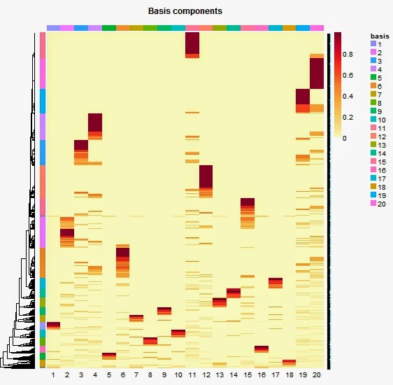
The above basis heatmap fills in the details for all 2218 respondents. As expected, the largest solid block is associated with the most chosen Chivas Regal also known as Basis #20. There I am in Basis #11 at the top with my Dewar's Only fellow drinkers. The top portion of heatmap is where most of the single brand users tend to be located, which is why there is so much yellow in this region outside of the dark reddish blocks. Toward the bottom of the heatmap is where you will find that small percentage purchasing many different brands. Since each basis component is associated with a particular brand, in order for a respondent to have acquired more than one brand they would need to belong to more than one cluster. Our more intense variety seekers fall toward the bottom and appear to have membership probabilities just below 0.2 for several basis components.

As I have already noted, little is gained by going from the original 21 brands to 20 basis components. Obviously, we would want considerable more rank reduction before we call it a segmentation. However, we did learn a good deal about how NMF decomposes a data matrix, and that was the purpose of this intuition building exercise. In a moment I will show the same analysis with rank equal to 5. For now, I hope that you can see how one could extract as many basis components as columns and reproduce each respondent's profile as a linear combination of those basis components. Can we do the same with fewer basis components and still reproduce the systematic portion of the data matrix (no one wants to overfit and reproduce noise in the data)?

By selecting 5 basis components I can demonstrate how NMF decomposes the sparse binary purchase data. Five works for this illustration, but the rank argument can be changed in the R code below to any value you wish. The above heatmap finds our Chivas Regal component, remember that 200 respondents drank nothing but Chivas Regal. It seems reasonable that this 9% should establish an additive component, although we can see that the row is not entirely yellow indicating that our Basis #3 includes a few more respondents than the 200 purists. Our second most popular brand, Dewar's, anchors Basis #2. The two Johnnie Walker offerings double up on Basis #4, and J&B along with Cutty Sark dominate Basis #5.  So far, we are discovering a brand defined decompose of the purchase data, except for the first basis component that represents the single malts. Though Other Brands is unspecified, all the single malts have very high coefficients on Basis #1.

Lastly, we should note that there is still a considerable amount of yellow in this heatmap, however, not nearly as much yellow as the first coefficient heatmap with the rank set to 20. If you recall the concept of simple structure from factor analysis, you will understand the role that yellow plays in the heatmap. We want variables to load on only one factor, that is, one factor loading for each variable to be as large as possible and the remaining loadings for the other factors to be as close to zero as possible. If factor loadings with a simple structure were shown in a heatmap, one would see a dark reddish block with lots of yellow.

We end with the heatmap for the 2218 respondents, remembering that there are only 484 unique profiles. NMF yields what some consider to be a soft clustering with each respondent assigned a number that behaves like a probability (i.e., ranges from 0 to 1 and sums to 1). This is what you see in the heatmap. Along the side you will find the dendrogram from a hierarchical clustering. If you preferred, you can substitute some other clustering procedure, or you can simply assign a hard clustering with each respondent assigned to the basis having the highest score. Of course, nothing is forcing a discrete representation upon us. Each respondent can be described as a profile of basis component scores, not unlike principal component or factor scores.

The underlying heterogeneity is revealed by this heatmap. Starting from the top, we find the Chivas Regal purist (Basis #3 with dark red in the third column and yellow everywhere else), then the single malt drinkers (Basis #1), followed by a smaller Johnny Walker subgroup (Basis #4) and a Dewar's cluster (Basis #2). Finally, looking only at those rows that have one column of solid dark red and yellow everywhere else, you can see the J&B-Cutty Sark subgroup (Basis #5). The remaining rows of the heatmap show considerably more overlap because these respondents' purchase profile cannot be reproduced using only one basis component.

Individual purchase histories are mixtures of types. If their purchases were occasion-based, then we might expect a respondent to act sometimes like one basis and other times like another basis (e.g., the block spans Basis #3 and #4 approximately one-third down from the top). Or, they may be buying for more than one person in the household. I am not certain if purchases intended as gifts were counted in this study.

Why not just run k-means or some other clustering method using the 21 binary variables without any matrix factorization? As long as distances are calculated using all the variables, you will tend to find a "buy-it-all" and a "don't-buy-many" cluster. In this case with so little brand variety, you can expect to discover a large segment with few purchases of more than one brand and a small cluster who purchases lots of brands. That is what Grun and Leisch report in their 2007 R News paper, and it is what you will find if you run that k-means using this data. I am not denying the one can "find" these two segments in the data. It is just not a very interesting story.

R Code for All Analysis in Post

# the data come from the bayesm package
library(bayesm)
data(Scotch)
 
library(NMF)
fit<-nmf(Scotch, 20, "lee", nrun=20)
coefmap(fit)
basismap(fit)
 
fit<-nmf(Scotch, 5, "lee", nrun=20)
basismap(fit)
coefmap(fit)
 
# code for sorting and printing
# the two factor matrices
h<-coef(fit)
library(psych)
fa.sort(t(round(h,3)))
w<-basis(fit)
wp<-w/apply(w,1,sum)
fa.sort(round(wp,3))
 
# hard clustering
type<-max.col(w)
table(type)
t(aggregate(Scotch, by=list(type), FUN=mean))

Created by Pretty R at inside-R.org